Technical
March / April 2025

Identifying Out-of-Trend Data In Stability Studies

Prasanth Sambaraju
Identifying Out-of-Trend Data In Stability Studies

Drug stability data that deviate from an expected trend when compared to other stability batches or historical data collected during stability studies are considered out-of-trend (OOT) results. According to the US Food and Drug Administration’s “Investigating Out-Of-Specification (OOS) Test Results for Pharmaceutical Production Guidance for Industry,” OOT results should be limited and scientifically justified.

However, the US FDA guidance does not specify the process for identifying OOT results in stability data 3. Different approaches have been historically used to identify OOT results, including:

  • Three consecutive results are outside the prescribed limits
  • The difference between consecutive results is outside of half the difference between the prior result and the specified limit
  • The current result is outside ± 5% of the initial result
  • The current result is outside ± 3% of the previous result
  • The current result is outside ± 5% of the mean of all the previous results

These approaches are easy to understand and implement. They also do not require different limits for each time point. The major disadvantage of these approaches is that they lack statistical basis 4, which raises questions about the reliability of these approaches to clearly and precisely detect OOT.

Methods for Detecting OOT Results

The following three methods are outlined and illustrated by the Pharmaceutical Research and Manufacturers of America (PhRMA) Chemistry, Manufacturing, and Control (CMC) Statistics and Stability Expert Teams for detecting OOT results 4, 5.

  • Regression control chart method
  • By-time-point method
  • Slope control chart method

The first method is suitable for both comparisons within-batch and between-batch comparisons, whereas the second and the third methods are only suitable for comparisons with other batches.

Regression Control Chart Method

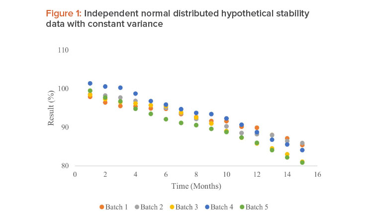
In the regression control chart method, data within a batch or data among batches are calculated. The control chart limits bracket the regression line along the length of the stability study. This method assumes that the data are normally and independently distributed with a constant variability across all time points, as shown in Figure 1. A common linear slope for all batches is also required for this method. For comparisons within a batch, a regression line is fit to the data for that batch.

For comparisons among batches, a regression line is fit to the historical data for the product, assuming a common slope but different intercepts for different batches. The fit obtained will provide an estimate of the intercepts, the slope, and the square root of the mean square error. A common slope estimate and standard error from the regression from historical batches can also be used. An estimate of the expected result at any given time point for a given batch is specified by the following equation:

Expected result = intercept + (slope × time)

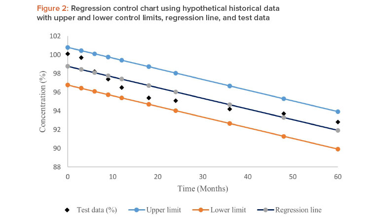
The control limits at a given time point are given by the expected result ± (k × s), where k is the multiplier obtained from normal quantiles at a desired level and s is the square root of the mean squared error from regression. These limits are also called Shewhart limits 5. Stability data points outside the control limits at a given time point are considered OOT, and such data points are investigated further 4. A regression control chart for hypothetical historical data with upper and lower limits and test data is shown in Figure 2.

Identifying Out-of-Trend Data In Stability Studies

By-Time-Point Method

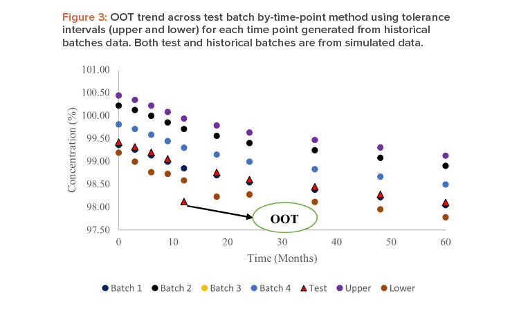
In this approach, data from historical batches are used to compute a tolerance interval for each stability time point. The tolerance interval can be based on the stability results or by using the difference from the initial stability result to minimize the effect of time zero differences among the tested batches. To calculate a tolerance interval, mean (x̅) and standard deviation (s) for each time point are calculated.

The intervals are then calculated as x̅ ± ks, where k is the multiplier value obtained from tables or approximation. The width of the interval depends on the number of historical batches and the levels of confidence and coverage desired, as shown in Figure 3. Data points outside these limits are considered OOT. The advantages of this method are that it requires no assumptions about the shape of degradation and it is used when different time points have variability4.

Slope Control Chart Method

For each time point, a least squares regression fit is generated that includes all data up to that time point. The slope estimate for each batch is used to find the overall slope and control limits. As the slopes are normally distributed, OOT limits for the slopes at each time point are obtained from the tolerance interval (x̅ ± ks), in which the value k is chosen to obtain the desired coverage. Further, x̅ and s are the mean and standard deviation of the historical slope values4.

Identifying Out-of-Trend Data In Stability Studies

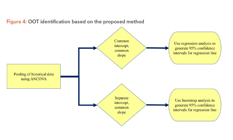
The goal of this article is to create a new method to identify OOT based on the regression control chart method. In the first step, data from all the historical batches are tested for pooling using analysis of covariance (ANCOVA). If the historical batches can be pooled using the common intercept and common slope (CICS) model, then regression analysis of data from historical batches is performed and the 95% confidence intervals (CI) for the regression line are obtained. If any data points from the test batch fall outside the 95% CI limit, the data are considered OOT.

If the historical batches can be pooled using the separate intercept and common slope (SICS) model, bootstrap analysis is performed on the historical data to generate 95% CI for the regression line. If any data points from the test batch fall outside the 95% CI limit, they are examined as OOT. This method cannot be applied if the data from historical batches cannot be pooled: In this case, the separate intercept and separate slope (SISS) model would be used for ANCOVA analysis. The schematic outline of this method is shown in Figure 4.

The 95% CI, for the dependent variable (yi) for a given independent variable (xi), is given by the following equation 6:

$$\begin{align} (mx_i + b) \pm t(\alpha, n - 2) \times S_{yx} \times \sqrt{\frac{1}{n} + \frac{(x_i - \bar{x})^2}{\sum_{i=1}^n (x_i - \bar{x})^2}} \tag{2} \end{align} $$2

Where m equals slope, b equals intercept, a equals significance level (0.05), n equals number of observations, and Syx equals the standard error of the predicted y value for each x in the regression. It is a measure of the amount of error in the prediction of y for an individual x. This value can be obtained by STEYX function in Microsoft Excel 7.

ANCOVA

A covariate is a variable that is not the variable of research interest, but may affect the dependent variable and its relationship with the independent variable. The effect of a covariate variable is controlled by changing the variance of dependent variables. It is also controlled by the relationship between the dependent variable and the covariate at different levels of variables being analysed.

ANCOVA analysis is a statistical method that involves combination of analysis of variance (ANOVA) and regression analysis for adjusting the linear effect of covariate. The main advantage of using ANCOVA is its ability to uncover variance changes of the dependent variable due to change in the covariate and to discriminate it from the changes in variance due to changes in the levels of the qualitative variable. ANCOVA reduces errors in dependent variables and increases analytical power 8.

Materials and Methods

Data in Table 1 reported by Mihalovits and Sándor containing eight batches of historical data and the ninth batch as test data were used to demonstrate this approach 5. The historical data were tested for pooling criteria using ANCOVA method in Microsoft Excel. Based on the model used for pooling historical data, 95% CIs for the regression line were obtained. Hypothetical data in Table 2 containing three historical batches and one test batch were used.

Data Pooling Using ANCOVA

The use of Microsoft Excel to test the equality of slopes and intercepts using ANCOVA for three batches was described by LeBlond  9. When the number of test batches is greater than three, the test for equality of slope and intercepts using Microsoft Excel was described by Sambaraju 10. In these tests, a significance level of 0.05 was used as the criterion for pooling. Based on ANCOVA analysis results, the SICS model was used to pool the data from historical batches.

Bootstrap Method

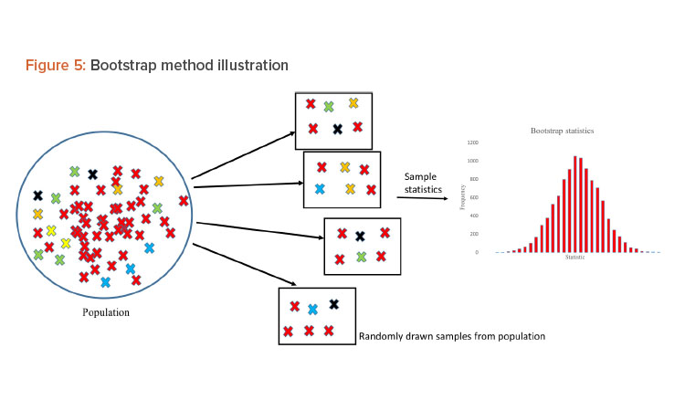
The bootstrap method was employed to generate 95% CIs for the regression line. The bootstrap method was introduced by Efron in 1979 to assess the statistical accuracy of the estimator 1. It is a computer-based resampling technique that uses new samples with repetition from original sample data to estimate the relevant properties of the population.

Identifying Out-of-Trend Data In Stability Studies

The main advantage of this technique is its simplicity, reliability, and ability to check the stability of results12. Figure 5 shows an illustration of the bootstrap method. The Visual Basic for Application (VBA) code to generate bootstrap samples in Microsoft Excel is included in Table 3. The CICS model was used based on the results obtained for pooling of historical data in Table 2 using the ANCOVA method in Microsoft Excel.

Results and Discussion

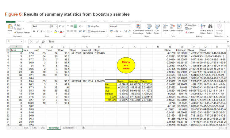
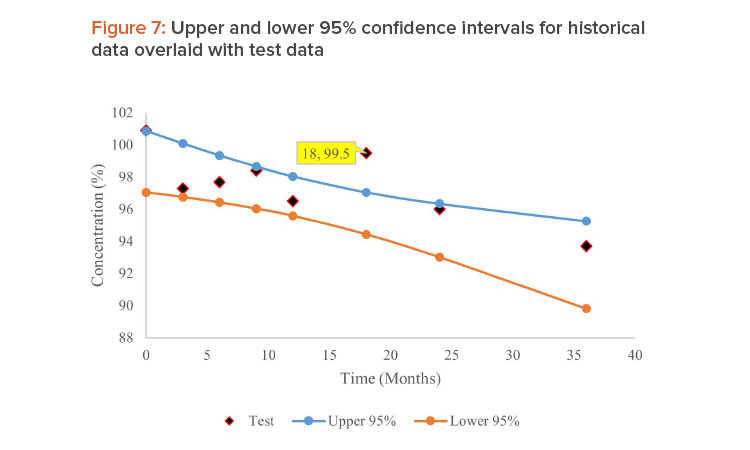
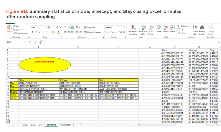
The results of summary statistics from bootstrap samples are shown in Figure 6. The 95% CIs for regression were generated using equation 2 and are shown in Figure 7. After the test data (ninth batch) were overlaid on this plot, data points that are outside the 95% CIs are considered as OOT. In this case, the 18-month time point data are considered as OOT. The results reported by Mihalovits and Sándor concluded that data from time points 9 to 36 months are OOT using Shewhart limits and data from the 18-month time point are OOT according to prediction limits and confidence limits. No data are OOT as per the tolerance limits method 5.

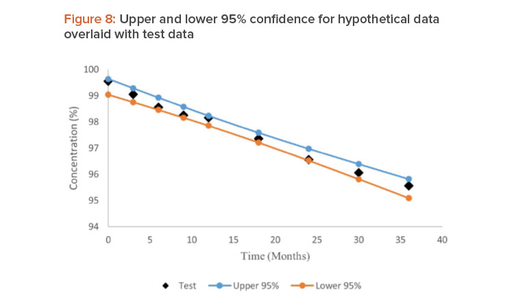
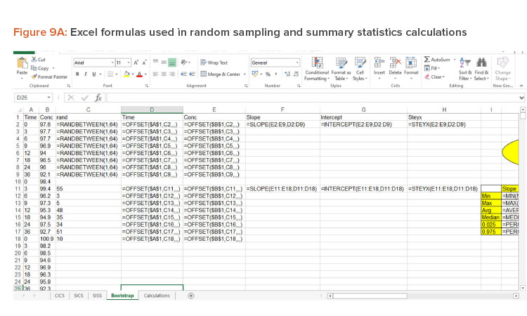
In case of hypothetical data, it can be observed that the test data points are within the 95% CIs, as shown in Figure 8. No test data point was considered as OOT. The Excel formula used in these calculations is shown in Figure 9.

Identifying Out-of-Trend Data In Stability Studies

Conclusion

Identifying OOT in stability studies is a challenge in the pharmaceutical industry. The historical methods used to identify OOT are not sensitive enough to identify a true OOT or may have high false-positive OOT results. The modified regression control chart method provides another statistically rigorous alternative approach that is not too complex and has limits that are not too narrow, unlike Shewhart limits.

This method can mitigate the incorrect use of tolerance intervals, which would widen the acceptance interval. This article provides a method for identifying OOT using Microsoft Excel with modest programming skills (see Figure 9A and 9B). This study also highlights the necessity of regulatory guidelines for identification of OOT results while performing stability data studies to enable a harmonized way of OOT identification. 11

Identifying Out-of-Trend Data In Stability Studies
Table 1: Historical stability data (Batches 1 to 8) and test data (Batch 9)
Time (month)Active drug (%)
 Batch 1Batch 2Batch 3Batch 4Batch 5Batch 6Batch 7Batch 8Batch 9
097.698.4100.998.798.8100.5100.3101.5100.9
397.799.498.295.897.596.599.7100.197.3
697.796.298.596.797.59698.699.597.7
996.997.394.697.598.996.398.399.698.4
129495.396.994.797.598.396.898.396.5
1896.594.996.393.796.594.196.795.299.5
249697.595.893.19692.596.397.196
3692.192.792.391.39289.593.993.893.7
Table 2: Hypothetical historical data (batches 1 to 3) and test data
Time (Months)Batch 1 (Conc %)Batch 2 (Conc %)Batch 3 (Conc %)Test (Conc %)
099.8099.6499.6199.55
399.3099.1499.1199.05
698.8098.6498.6198.55
998.3098.1498.1198.05
1297.8097.6497.6197.55
1897.3097.1497.1197.05
2496.8096.6496.6196.55
3096.3096.1496.1196.05
3695.8095.6495.6195.55
Table 3: Excel visual basic code to generate bootstrap resamples
Sub bootstrap()
Dim i As Long
Application.ScreenUpdating = False
Application.Calculation = xlCalculationManual
On Error Resume Next
'In case if cells in Range("N2", Range("N2").End(xlDown).End(xlToRight)) are empty
Range("N2", Range("N2").End(xlDown).End(xlToRight)).ClearContents
'To create bootstrap
For i = 1 To 10000
  Application.StatusBar = "Processing " & i & " of 10000"
  Range("F2:H2").Copy
  Range("N" & Rows.Count).End(xlUp).Offset(1, 0).PasteSpecial (xlPasteValues)
  Range("Q" & Rows.Count).End(xlUp).Offset(1, 0).Value = Range("C2").Value & "-" & Range("C3").Value
  & "-" & Range("C4").Value & "-" & Range("C5").Value & "-" & Range("C7").Value & "-" & Range("C9").Value & "-" &
  Range("C5").Value
  'Trace slope, intercept & STEYX values in case if there is any error
Next i
Application.ScreenUpdating = True
Application.Calculation = xlCalculationAutomatic
End Sub
        

Unlock Access to Member-Only Content

Complete the form below to get exclusive access to Member-only content. Each issue of Pharmaceutical Engineering magazine features thought-provoking content that is available to Members only, but NOW we're giving you exclusive access to see what you've been missing out on.

Name
Address

By completing this form, you consent to have your information provided to the third-party sponsor of this content and may use your information to provide information about relevant products, services, and other opportunities which may be of interest to you . ISPE will store your information in a secure environment and may use your information to provide information about relevant products, services, and other opportunities which may be of interest to you. You may unsubscribe from these ISPE communications at any time. For more information or to unsubscribe, review our Privacy Policy or contact us at ask@ispe.org.

CAPTCHA
This question is for testing whether or not you are a human visitor and to prevent automated spam submissions.
QA